fancy ggplot
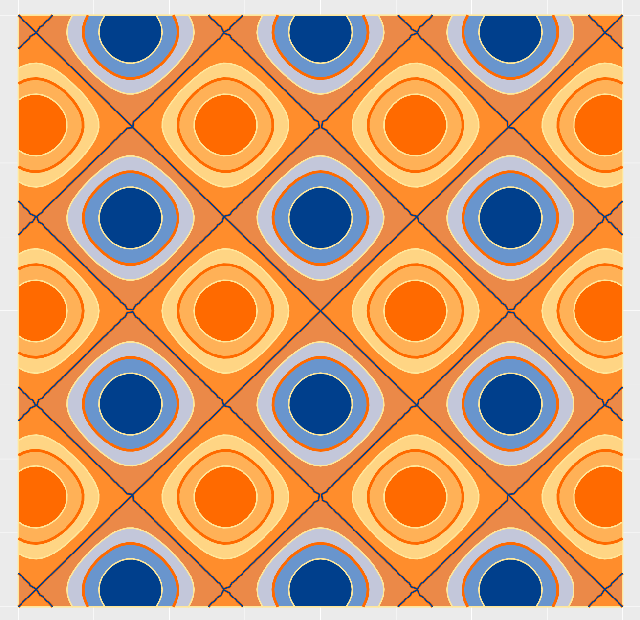
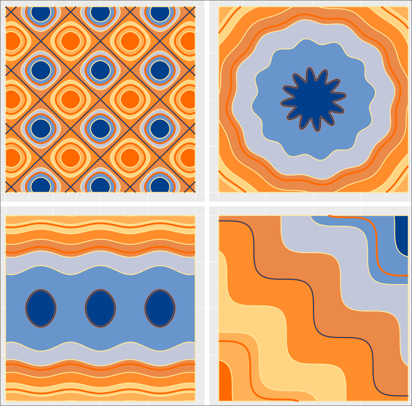
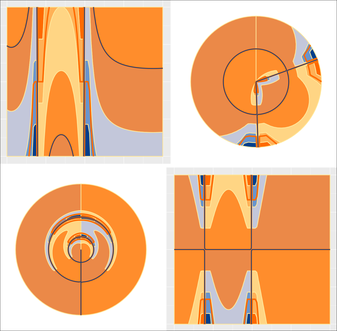
Zuerst haben wir einfach nur einen schönen Plot. Dieser visualiseiert 4 unterschiedliche Funktionen auf ein ähnliche Art und weise.
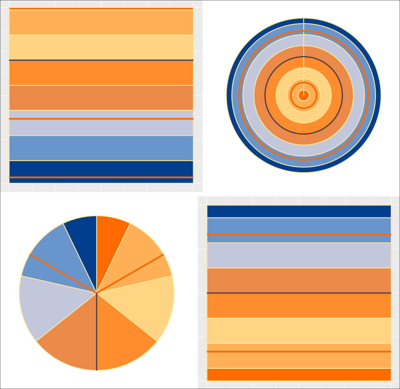
In unserem Zweiten Plott stellen wir die Konstante Funktion 2 dar. Wir haben die klarsten visualisierung oben links als linearen plot. Oben rechts haben wir ein polar coordinate plot, bei dem der abstand konstant gehalten wird und unten links haben wir einen polar plot bei dem der winkel konstant gehalten wird. Unten rechts haben wir abschliessend einen plot mit einer Multiplikation der konstante.
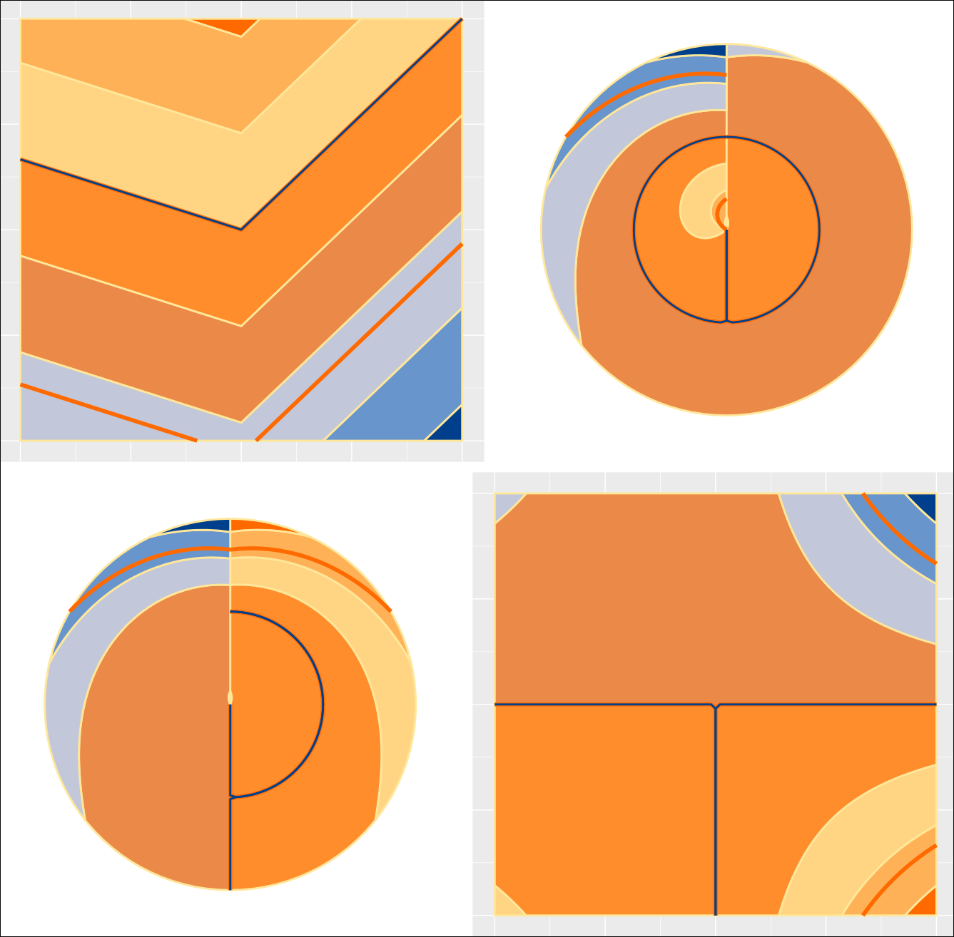
Hier haben wir die selben vie plots aber mit einer Funktion die im Kern den absoluten wert wieder spiegelt mit etwas abflachen und verschieben.
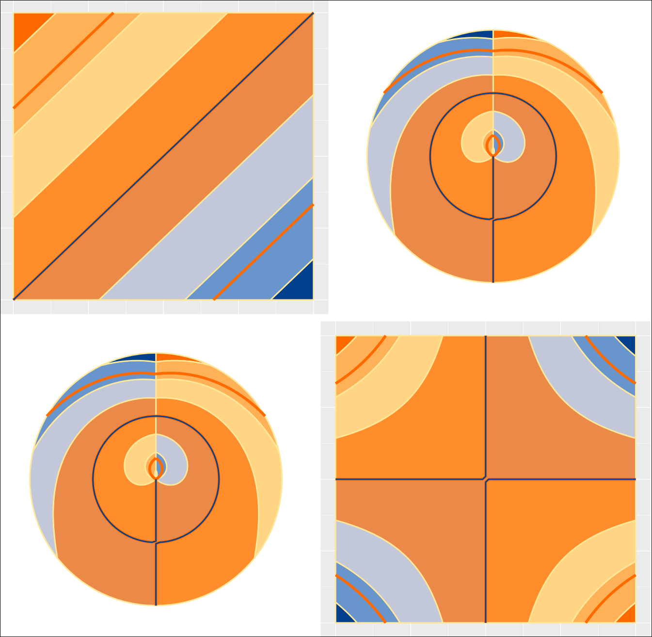
Hier haben wir die einfachste nicht konstante funkction. Wir haben einfach f(x) = x.
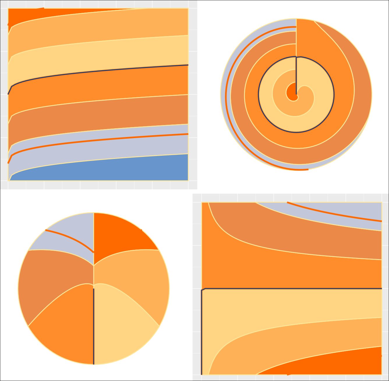
Überraschend ästhetisch ist die dritte Wurzel nicht mehr und nicht weniger sehen wir hier.
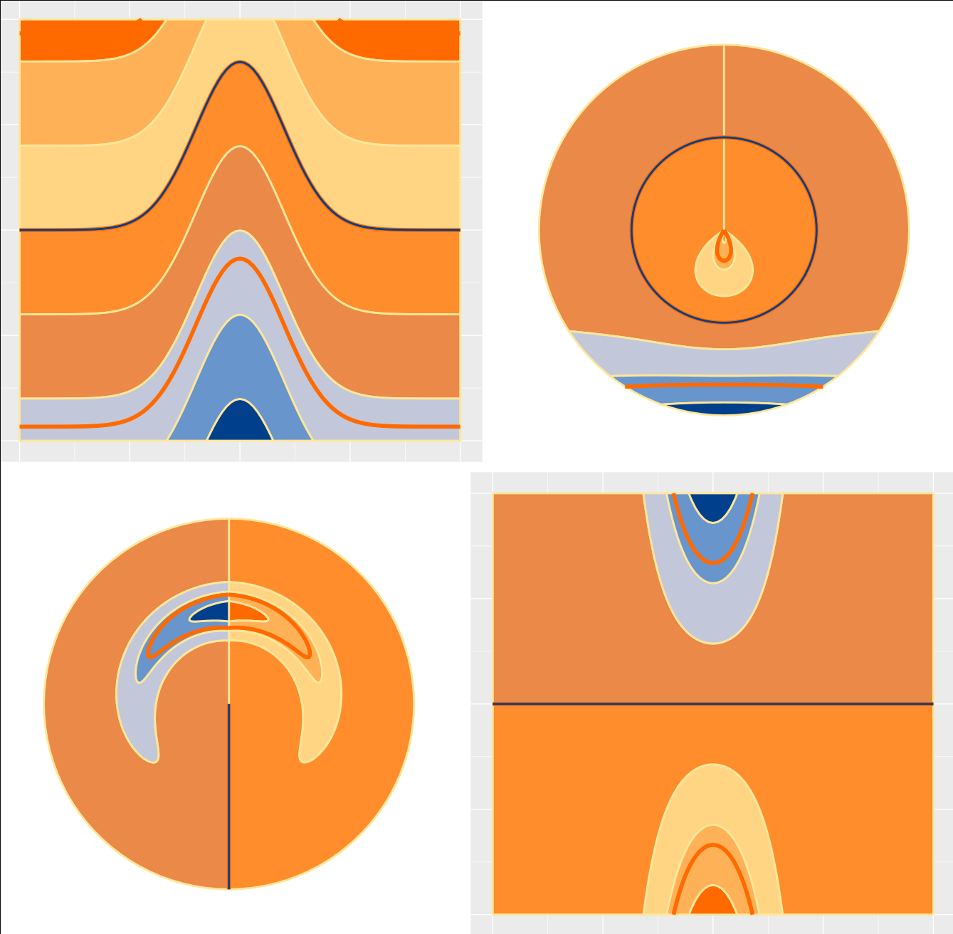
Auch die normalverteilung kann hier dargestellt werden. Und auch diese ist hübsch macht aber macht teilweise ein KI eindruck :(
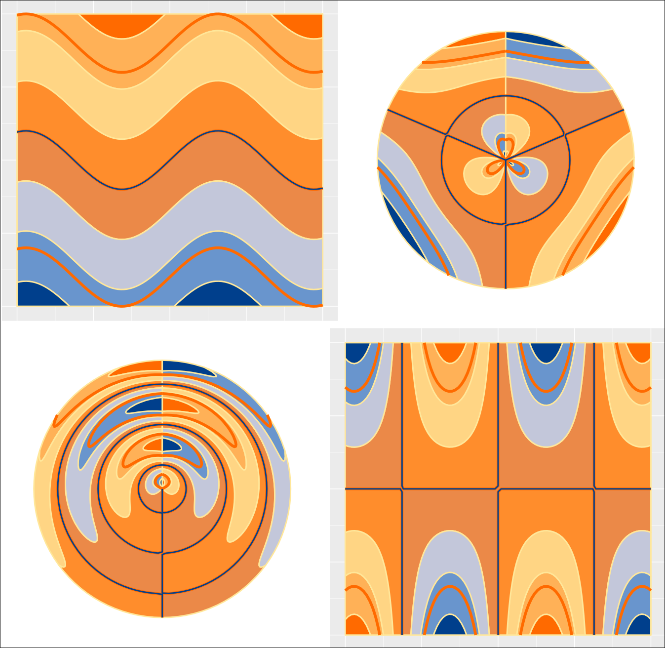
Sinus ist auch vertreten.
Und die gamma funktion mag zwar mathematisch schön sein aber ist etwas zu kompliziert um saubere plotts zu generieren.
R-Script
library(tidyverse)
library(patchwork)

grid <- expand.grid(x = -50:50 / 10, y = -50:50 / 10) %>%
  mutate(z = x + y)

spec <- c("orange", "green", "black")

spec <- c(
  "königs blau" = "#003F8C", # deep royal blue
  "knalliges orange" = "#FF6A00", # vivid orange
  "pastell gelb" = "#FFE79A", # pastel yellow
  "hell grau mit viel blau anteil" = "#B9D7FF" # light gray-blue
)

cols_ramp <- grDevices::colorRampPalette(c(
  spec[2],
  spec[3],
  spec[2],
  spec[4],
  spec[1]
))

bins <- 8
cols_bins <- cols_ramp(bins)

# front image
grid %>%
  ggplot(aes(x = x, y = y, z = cos(x)^2 + sin(y)^2)) +
  geom_contour_filled(
    bins = bins,
    color = spec[3],
    show.legend = FALSE,
    linewidth = 1
  ) +
  geom_contour(bins = 4, color = spec[2], linewidth = 2) +
  geom_contour(bins = 2, color = spec[1], linewidth = 1) +
  scale_fill_manual(values = cols_bins) +
  theme(
    axis.text.x = element_blank(),
    axis.ticks.x = element_blank(),
    axis.text.y = element_blank(),
    axis.ticks.y = element_blank()
  ) +
  labs(x = NULL, y = NULL)

fancy_contour <- function() {
  list(
    geom_contour_filled(
      bins = bins,
      color = spec[3],
      show.legend = FALSE,
      linewidth = 1
    ),
    geom_contour(bins = 4, color = spec[2], linewidth = 2),
    geom_contour(bins = 2, color = spec[1], linewidth = 1),
    scale_fill_manual(values = cols_bins),
    theme(
      axis.text.x = element_blank(),
      axis.ticks.x = element_blank(),
      axis.text.y = element_blank(),
      axis.ticks.y = element_blank(),
      # plot.margin = margin(0, 0, 0, 0),
      # panel.spacing = unit(0, "pt"),
      # aspect.ratio = 1
    ),
    labs(x = NULL, y = NULL)
  )
}


a <- grid %>%
  ggplot(aes(x = x, y = y, z = cos(x)^2 + sin(y)^2)) +
  fancy_contour()

b <- grid %>%
  ggplot(aes(x = x, y = y, z = -x^2 - y^2 + 2 + sin(atan2(y, x) * 12))) +
  fancy_contour()

c <- grid %>%
  ggplot(aes(x = x, y = y, z = cos(x * 2) - y^2)) +
  fancy_contour()

d <- grid %>%
  ggplot(aes(x = x, y = y, z = sin(x - y) + x + y)) +
  fancy_contour()

(a + b) / (c + d)

# 1-different
func <- function(x) x

fancy_plot <- function(func) {
  lin <- grid %>%
    ggplot(aes(x = x, y = y, z = func(x) - y)) +
    fancy_contour()

  mul <- grid %>%
    ggplot(aes(x = x, y = y, z = func(x) * y)) +
    fancy_contour()

  pol1 <- grid %>%
    ggplot(aes(x = x, y = y, z = func(x) * y)) +
    fancy_contour() +
    # xlim(c(-2,2)) +
    coord_radial(expand = FALSE)

  pol2 <- grid %>%
    ggplot(aes(x = x, y = y, z = x * func(y))) +
    fancy_contour() +
    # ylim(c(-2,2)) +
    coord_radial(expand = FALSE)

  (lin + pol1) / (pol2 + mul)
}

# 2-constant
fancy_plot(function(x) 2)

# 3-shifted-abs
fancy_plot(function(x) abs(x) * (2 + sign(x)) / 3)

# 4-linear
fancy_plot(function(x) x)

# 5-root
fancy_plot(function(x) x^(1 / 3))

# 6-binom
fancy_plot(function(x) dnorm(x) * 10)

# 7-sin
fancy_plot(function(x) sin(x))

# 8-gamma
fancy_plot(function(x) pmin(pmax(gamma(x / 3 + 0.001), -10), 10))

fancy_plot(function(x) x^3)